Lasso简介
LASSO(Least Absolute Shrinkage and Selection Operator)是线性回归的一种缩减方式,通过引入$L_1$惩罚项,实现变量选择和参数估计。
$$\sum_{i=1}^{N}\left(y_{i}-\beta_{0}+\sum_{j=1}^{p} x_{i j} \beta_{j}\right)^{2}+\lambda \sum_{j=1}^{p}\left|\beta_{j}\right|$$
R示例
简单的建模过程主要包括:
- 数据切分、清洗
- 建模,使用R的
glmnet包即可实现lasso - 评估,分类常使用混淆矩阵、ROC(使用
ROCR包),数值型预测常使用MAPE
以下用简单的数据集实现Lasso-LR:
这是由真实的医学数据抽样得到的一份demo数据,x1-x19分别代表不同的基因或者染色体表现数据,Y代表病人是否患有某种疾病。(由于数据敏感,因此都用$X_i$代替。)1
2
3rm(list=ls())
library(data.table)
dat_use <- fread('demo_data.csv',header = T)
1 | head(dat_use) |
数据预处理
首先将类别型变量转为哑变量,借助caret的dummyVars函数可以轻松获取哑变量1
2
3
4
5
6
7
8
9
10
11
12library(caret)
# Genotype 为数据中多类型的类别型变量,其他例如Age和Gender为二值0-1变量,无需再转换
# 首先将类别型变量转为facor类型
names_factor <- c('Genotype')
dat_use[, (names_factor) := lapply(.SD, as.factor), .SDcols = names_factor]
# 抽取出类别型变量对应的哑变量矩阵
dummyModel <- dummyVars(~ Genotype,
data = dat_use,
sep = ".")
dat_dummy <- predict(dummyModel, dat_use)
# 合并哑变量矩阵,并删除对应原始数据列
dat_model <- cbind(dat_use[,-c(names_factor),with=F],dat_dummy)
1 | head(dat_dummy) |
切分数据集1
2
3
4
5
6
7
8
9
10
11
12
13
14
15
16
17# 设置随机数种子,便于结果重现
set.seed(1)
# split data
N <- nrow(dat_model)
test_index <- sample(N,0.3*N)
train_index <- c(1:N)[-test_index]
test_data <- dat_model[test_index,]
train_data <- dat_model[train_index,]
# 指定因变量列,
y_name <- 'y'
thedat <- na.omit(train_data)
y <- c(thedat[,y_name,with=F])[[1]]
x <- thedat[,c(y_name):=NULL]
x <- as.matrix(x)
# normalize(此步骤可省略,因为glmnet默认会标准化后建模,再返回变换后的真实系数)
# pp = preProcess(x,method = c("center", "scale"))
# x <- predict(pp, x)
建模
1 | library(glmnet) |
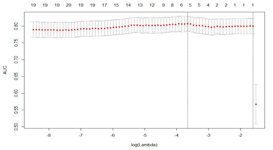
可以看到压缩到5个变量时AUC最大,对应 $log(lambda)=-3.67$,抽取出对应5个变量的模型系数如下1
2
3
4
5
6
7
8
9
10
11
12# log(fit_cv$lambda.min)=-3.67
get_coe <- function(the_fit,the_lamb){
Coefficients <- coef(the_fit, s = the_lamb)
Active.Index <- which(Coefficients != 0)
Active.Coefficients <- Coefficients[Active.Index]
re <- data.frame(rownames(Coefficients)[Active.Index],Active.Coefficients)
re <- data.table('var_names'=rownames(Coefficients)[Active.Index],
'coef'=Active.Coefficients)
# 计算系数的指数次方,表示x每变动一个单位对y的影响倍数
re$expcoef <- exp(re$coef)
return(re[order(expcoef)])
}
1 | get_coe(fit_cv,fit_cv$lambda.min) |
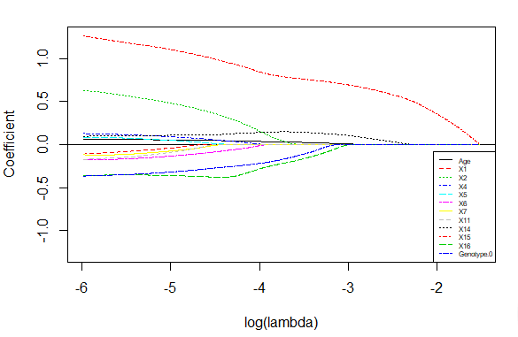
但医学上经常需要看每个变量在不同惩罚参数lambda下的压缩程度,从而结合实际背景进一步判别有效的影响因素,因此可借助以下图像进行分析,可以看到x15对y的影响最大(此去省略1000字)1
2
3
4
5
6
7
8
9
10
11
12
13
14
15
16
17
18
19
20get_plot<- function(the_fit,the_fit_cv,the_lamb,toplot = seq(1,50,2)){
Coefficients <- coef(the_fit, s = the_lamb)
Active.Index <- which(Coefficients != 0)
coeall <- coef(the_fit, s = the_fit_cv$lambda[toplot])
coe <- coeall[Active.Index[-1],]
ylims=c(-max(abs(coe)),max(abs(coe)))
sp <- spline(log(the_fit_cv$lambda[toplot]),coe[1,],n=100)
plot(sp,type='l',col =1,lty=1,
ylim = ylims,ylab = 'Coefficient', xlab = 'log(lambda)')
abline(h=0)
for(i in c(2:nrow(coe))){
lines(spline(log(the_fit_cv$lambda[toplot]),coe[i,],n=1000),
col =i,lty=i)
}
legend("bottomright",legend=rownames(coe),col=c(1:nrow(coe)),
lty=c(1:nrow(coe)),
cex=0.5)
}
# 传入最优lambda-1,从而保留更多变量
get_plot(fit,fit_cv,exp(log(fit_cv$lambda.min)-1))
评估
对于分类模型,最常用的评估指标莫过于AUC值了,使用ROCR包可获取AUC值,为了多维度的评估,将混淆矩阵,和各种recall/accuracy指标加入其中。1
2
3
4
5
6
7
8
9
10
11
12
13
14
15
16
17
18
19
20
21
22
23
24
25
26
27
28
29
30
31
32
33
34
35
36
37
38
39
40library(ROCR)
get_confusion_stat <- function(pred,y_real,threshold=0.5){
# auc
tmp <- prediction(as.vector(pred),y_real)
auc <- unlist(slot(performance(tmp,'auc'),'y.values'))
# statistic
pred_new <- as.integer(pred>threshold)
tab <- table(pred_new,y_real)
if(nrow(tab)==1){
print('preds all zero !')
return(0)
}
TP <- tab[2,2]
TN <- tab[1,1]
FP <- tab[2,1]
FN <- tab[1,2]
accuracy <- round((TP+TN)/(TP+FN+FP+TN),4)
recall_sensitivity <- round(TP/(TP+FN),4)
precision <- round(TP/(TP+FP),4)
specificity <- round(TN/(TN+FP),4)
# 添加,预测的负例占比(业务解释:去除多少的样本,达到多少的recall)
neg_rate <- round((TN+FN)/(TP+TN+FP+FN),4)
re <- list('AUC' = auc,
'Confusion_Matrix'=tab,
'Statistics'=data.frame(value=c('accuracy'=accuracy,
'recall_sensitivity'=recall_sensitivity,
'precision'=precision,
'specificity'=specificity,
'neg_rate'=neg_rate)))
return(re)
}
# 结合数据预处理部分,得到模型在测试集上的表现
get_eval <- function(data,theta=0.5,the_fit=fit,the_lamb=fit_cv$lambda.min){
thedat_test <- na.omit(data)
y <- c(thedat_test[,y_name,with=F])[[1]]
x <- thedat_test[,-c(y_name),with=F]
x <- as.matrix(x)
pred <- predict(the_fit,newx=x,s=the_lamb,type = 'response')
print(get_confusion_stat(pred,y, theta))
}
1 | # get_eval(train_data) 篇幅原因不再展示训练集的拟合效果 |
可以看到模型在测试集上的表选比较不错,AUC值达到0.84,不过在specificity上表现欠佳,说明在负样本上的召回较差(52个负样本,只预测对了20个)。